
According to Wikipedia, Bayesian optimization (BO) is a sequential design strategy for global optimization of black-box functions that do not require derivatives.
Study Objective
In this post, we will:
Review optimization algorithms. Compare Bayesian optimization with gradient descent.
Understand the process of Bayesian optimization.
Write a simple Bayesian optimization algorithm from scratch.
Use BO not from scratch.
Optimization
Optimization is to find the global max or min from the function. Besides BO, we also use grid search, random search and gradient descent. The first two can be used on any function if computation power is not the problem. The third is used only if the function is convex and derivative. Bayesian optimization has no such limitations. However, the function is supposed to be smooth and continuous, otherwise, I would recommend grid search and random search.
Process
I think the whole process can be demonstrated as the following trinity:
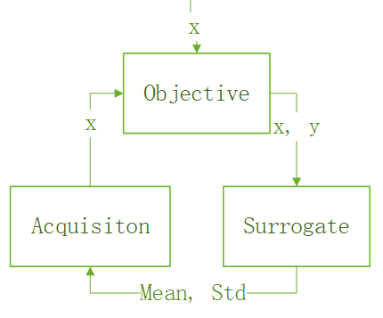
Here the objective function is the black function that we optimize. It produces samples (x, y). Usually, it is very costly to run the objective function, such that we introduce a surrogate function to predict the objective function. The prediction is mean and standard deviation of the objective function, which are used by the acquisition function in searching for the next x to explore or exploit. The next x is then consumed by the objective function. The loop goes on until the max or min is found.
The surrogate function is usually the Gaussian process regressor while the acquisition function has many options. They are:
- Probability of Improvement (PI).
- Expected Improvement (EI).
- Upper/Lower Confidence Bound (LCB/UCB).
Here we only focus on what we use, the UCB, the most straightforward one. If we ignore weight, UCB can be written as:
𝑈𝐶𝐵(𝑥)=𝜇(𝑥)+𝜎(𝑥)
𝑥=argmax 𝑈𝐶𝐵(𝑥)
We do all of this inside the search space.
The whole process:
- Initiate x with the min and max of the search space.
- Calculate y using x and objective function.
- Fit the surrogate function.
- Find new x using the acquisition function.
- Go to 1
Python Code
Let’s first define and plot the objective function as following:
1 | def objective(x): |
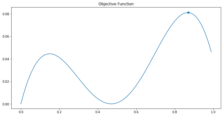
Here the maximum (x=0.87, y= 0.0811051) is also plotted as a blue point.
Now, this function is non-convex, thus gradient descent cannot be used. We use BO. The surrogate function is the Gaussian process regressor and UCB is used as the acquisition function.
1 | #uppper confidence bound (UCB) |
Code for the whole process
1 | #step 0 Initiate x with the min and max of the search space. |
Step 0:
In step 0, we simply produce two sample x=0 and x=1.
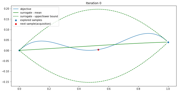
Iteration 0:
In iteration 0, the two samples are used by the surrogate function to generate mean and std(green). The acquisition function finds the max UCB when x=0.53(red). Objective(0.53) is 0.00359934. Now a new point (0.53, 0.00359934) is found. We give the three points to iteration 1.
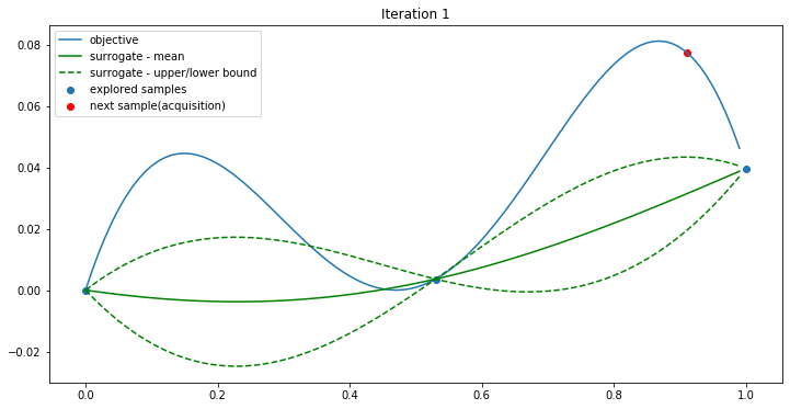
Iteration 1:
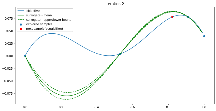
Iteration 2:
Iteration 3:
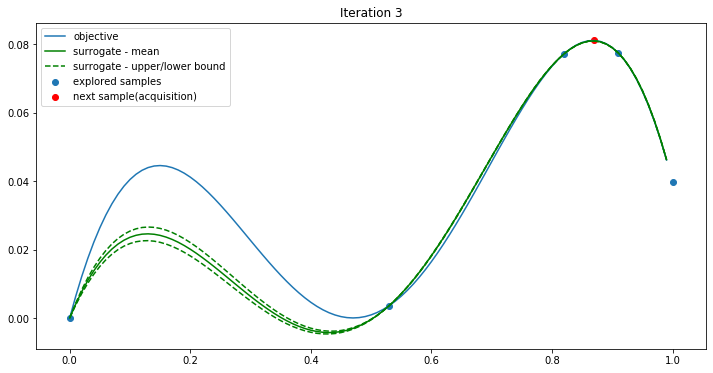
The new point(red) here is (0.53, 0.00359934) and it is just the max. We can see that BO can find the optimum in just 4 iterations. And we call the objective function only 6 times. If we use the grid search, that will be 100 times.
The complete version of the code can be found here:
https://github.com/EricWebsmith/machine_learning_from_scrach/blob/master/bayesian_optimization.ipynb
Bayesian Optimization not from scratch
There are many tools for BO. One of them is Hyperopt. The following is just a simple demonstration of that.
1 | from hyperopt import fmin, tpe, hp |