Gradient Boosting Regression from Scratch

Word count: 2.2kReading time: 13 min

 2020/04/12   Share

Gradient Boosting (GB) algorithm trains a series of weak learners and each focuses on the errors the previous learners have made and tries to improve it. Together, they make a better prediction.

According to Wikipedia, Gradient boosting is a machine learning technique for regression and classification problems, which produces a prediction model in the form of an ensemble of weak prediction models, typically decision trees. It builds the model in a stage-wise fashion as other boosting methods do, and it generalizes them by allowing optimization of an arbitrary differentiable loss function.

Prerequisite

1. Linear regression and gradient descent
2. Decision Tree

After studying this post, you will be able to:

1. Explain gradient boosting algorithm.
2. Explain gradient boosting regression algorithm.
3. Write a gradient boosting regressor from scratch

The algorithm

The following plot illustrates the algorithm.

Gradient Boosting Regression

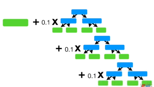
(Picture taken from Youtuber StatQuest with Josh Starmer)

From the plot above, the first part is a stump, which is the average of y. We then add several trees to it. In the following trees, the target is not y. Instead, the target is the residual or the true value subtract previous prediction.

$residual=true\_value - previous\_prediction$

That is why we say in Gradient Boosting trains a series of weak learners, each focuses on the errors of the previous one. The residual predictions are multiplied by the learning rate (0.1 here) before added to the average.

The Steps

Step 1: Calculate the average of y. The average is also the first estimation of y:

$\bar{y}=\frac{1}{n} \sum_{i=1}^{n}y_i$ $F_0(x)=\bar{y}$

Step 2 for m in 1 to M:

Step 2.1: Compute so-call pseudo-residuals:
$r_{im}=y_i-F_{m-1}(x_i)$
Step 2.2: Fit a regression tree $t_m(x)$ to pseudo-residuals and create terminal regions (leafs) $R_{jm}$ for $j=1...Jm$
Step 2.3: For each leaf of the tree, there are $p_j$ elements, compute $\gamma$ as the following equation.

$\gamma_{im}=\frac{1}{p_j} \sum_{x_i \in R_{jm}} r_{im}$

(In practice, the regression tree will do this for us.)
Step 2.4: Update the model with learning rate $\alpha$:
$F_m(x)=F_{m-1}+\alpha\gamma_m$

Step 3. Output $F_M(x)$

In practise the regression tree will average the leaf for us. Thus, Step 2.2 and 2.3 can be combined into one step. And the steps can be simplified:

New The Steps

Step 1: Calculate the average of y. The average is also the first estimation of y:

$\bar{y}=\frac{1}{n} \sum_{i=1}^{n}y_i$ $F_0(x)=\bar{y}$

Step 2 for m in 1 to M:

Step 2.1: Compute so-call pseudo-residuals: $r_{im}=y_i-F_{m-1}(x_i)$
Step 2.2: Fit a regression tree $t_m(x)$ to pseudo-residuals
Step 2.3: Update the model with learning rate $\alpha$:
$F_m(x)=F_{m-1}+\alpha t_m(x)$

Step 3. Output

$F_M(x)$

(Optional) From Gradient Boosting to Gradient Boosting Regression

The above knowledge is enough for writing BGR code from scratch. But I want to explain more about gradient boosting. GB is a meta-algorithm that can be applied to both regression and classification. The above one is only a specific form for regression. In the following, I will introduce the general gradient boosting algorithm and deduce GBR from GB.

Let’s first look at the GB steps

The Steps

Input: training set $\{(x_i, y_i)\}_{i=1}^{n}$ , a differentiable loss function $L(y, F(x))$ , number of iterations M

Algorithm:

Step 1: Initialize model with a constant value:

$F_0(x)=\underset{\gamma}{\operatorname{argmin}}\sum_{i=1}^{n}L(y_i, \gamma)$

Step 2 for m in 1 to M:

Step 2.1: Compute so-call pseudo-residuals:

$r_{im}=-[\frac{\partial L(y_i, F(x_i))}{\partial F(x_i)}]_{F(x)=F_{m-1}(x)}$

Step 2.2: Fit a weak learner $h_m(x)$ to pseudo-residuals. and create terminal regions $R_{jm}$ , for $j=1...J_m$
Step 2.3: For each leaf of the tree, compute $\gamma$ as following equation.

$\gamma_{jm}=\underset{\gamma}{\operatorname{argmin}}\sum_{x_i \in R_{jm}}^{n}L(y_i, F_{m-1}(x_i)+\gamma)$

Step 2.4: Update the model with learning rate $\alpha$: $F_m(x)=F_{m-1}+\alpha\gamma_m$

Step 3. Output $F_M(x)$

To deduce the GB to GBR, I simply define a loss function and solve the loss function in step 1, 2.1 and 2.3. We use sum of squared errror(SSE) as the loss function:

$L(y, \gamma)=\frac{1}{2}\sum_{i=1}^{n}(y_i-\gamma)^2$

For step 1:

Because SSE is a convex and at the lowest point where the derivative is zero, we have the following:

$\frac{\partial L(y, F_0)}{\partial F_0}=\frac{\partial \frac{1}{2}\sum_{i=1}^{n}(y_i-F_0)^2}{\partial F_0} =\sum_{i=1}^{n} (y_i-F_0)=0$

Thus, we have:

$F_0=\frac{1}{n}\sum_{i=1}^{n}y_i$

For step 2.1:

$r_{im}=-[\frac{\partial L(y_i, F(x_i))}{\partial F(x_i)}]_{F(x)=F_{m-1}(x)}$ $=-[\frac{\partial \frac{1}{2}\sum_{i=1}^{n}(y_i-F_{m-1}(x_i))^2)}{\partial F_{m-1}(x_i)}]_{F(x)=F_{m-1}(x)}$

(The chain rule)

$=--2*\frac{1}{2}(y_i-F_{m-1}(x_i))$ $=y_i-F_{m-1}(x_i)$

For step 2.3:

Similarly, the result is:

$\gamma_{jm}=\frac{1}{p_j}\sum_{x_i \in R_j}r_{im}$

Code

Let’s first import the modules.

import pandas as pd
from sklearn.tree import DecisionTreeRegressor
from sklearn.datasets import load_boston
import numpy as np
import matplotlib.pyplot as plt

import graphviz 
from sklearn import tree

And load data.

df=pd.DataFrame()
df['name']=['Alex','Brunei','Candy','David','Eric','Felicity']
df['height']=[1.6,1.6,1.5,1.8,1.5,1.4]
df['gender']=['male','female','female','male','male','female']
df['weight']=[88, 76, 56, 73, 77, 57]
display(df)

X=df[['height','gender']].copy()
X.loc[X['gender']=='male','gender']=1
X.loc[X['gender']=='female','gender']=0
y=df['weight']
display(X)

n=df.shape[0]

The data is display as:

name	height	gender	weight
Alex	1.6	male	88
Brunei	1.6	female	76
Candy	1.5	female	56
David	1.8	male	73
Eric	1.5	male	77
Felicity	1.4	female	57

And X is:

height	gender
1.6	1
1.6	0
1.5	0
1.8	1
1.5	1
1.4	0

Step 1 Average

#now let's get started
learning_rate=0.2
loss = [0] * 6
residuals = np.zeros([6,n])
predictoin = np.zeros([6,n])
#calculation
average_y=y.mean()
predictoin[0] = [average_y] * n
residuals[0] = y - predictoin[0]
df['$f_0$']=predictoin[0]
df['$r_0$']=residuals[0]
display(df)
loss[0] = np.sum(residuals[0] ** 2)
trees = []

The average and residuals are as following:

	name	height	gender	weight	𝑓0	𝑟0
0	Alex	1.6	male	88	71.166667	16.833333
1	Brunei	1.6	female	76	71.166667	4.833333
2	Candy	1.5	female	56	71.166667	-15.166667
3	David	1.8	male	73	71.166667	1.833333
4	Eric	1.5	male	77	71.166667	5.833333
5	Felicity	1.4	female	57	71.166667	-14.166667

In the first step, we calculate the average 71.2 as the initial prediction. The pseudo residuals are 16.8, 4.8, etc.

Step 2 For Loop

We define each iteration as following and we will call it from i=0 to 5.

def iterate(i):
    t = DecisionTreeRegressor(max_depth=1)
    t.fit(X,residuals[i])
    trees.append(t)
    #next prediction, residual
    predictoin[i+1]=predictoin[i]+learning_rate * t.predict(X)
    residuals[i+1]=y-predictoin[i+1]
    loss[i+1] = np.sum(residuals[i+1] ** 2)
    
    df[f'$\gamma_{i+1}$']=t.predict(X)
    df[f'$f_{i+1}$']=predictoin[i+1]
    df[f'$r_{i+1}$']=residuals[i+1]
    
    display(df[['name','height','gender','weight',f'$f_{i}$',f'$r_{i}$',f'$\gamma_{i+1}$',f'$f_{i+1}$',f'$r_{i+1}$']])
    
    dot_data = tree.export_graphviz(t, out_file=None, filled=True, rounded=True,feature_names=X.columns) 
    graph = graphviz.Source(dot_data) 
    display(graph)

Iteration 0

	name	height	gender	weight	𝑓0	𝑟0	𝛾1	𝑓1	𝑟1
0	Alex	1.6	male	88	71.166667	16.833333	8.166667	72.800000	15.200000
1	Brunei	1.6	female	76	71.166667	4.833333	-8.166667	69.533333	6.466667
2	Candy	1.5	female	56	71.166667	-15.166667	-8.166667	69.533333	-13.533333
3	David	1.8	male	73	71.166667	1.833333	8.166667	72.800000	0.200000
4	Eric	1.5	male	77	71.166667	5.833333	8.166667	72.800000	4.200000
5	Felicity	1.4	female	57	71.166667	-14.166667	-8.166667	69.533333	-12.533333

In Iteration 0, we first train a tree using residuals_0. This tree tells us that males are higher than females, each male should add 8.167 kg, each female subtracts -8.167 kg. The result of the tree is $\gamma$ here. But, we want to take just a small step a time, so we multiply the learning rate $\alpha=0.2$ . Thus, the new prediction is $prediction=prediction+\alpha\gamma$ . That is to say, for each male, he will add $8.167*0.2=1.6334$ kg. For each female, she will lose $-8.167*0.2=-1.6334$ kg. Finally, the males are predicted 72.8 kg and females 69.5.

Iteration 1

	name	height	gender	weight	𝑓1	𝑟1	𝛾2	𝑓2	𝑟2
0	Alex	1.6	male	88	72.800000	15.200000	7.288889	74.257778	13.742222
1	Brunei	1.6	female	76	69.533333	6.466667	7.288889	70.991111	5.008889
2	Candy	1.5	female	56	69.533333	-13.533333	-7.288889	68.075556	-12.075556
3	David	1.8	male	73	72.800000	0.200000	7.288889	74.257778	-1.257778
4	Eric	1.5	male	77	72.800000	4.200000	-7.288889	71.342222	5.657778
5	Felicity	1.4	female	57	69.533333	-12.533333	-7.288889	68.075556	-11.075556

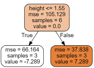
In iteration 1, we firstly train a tree using residuals_1. This tree tells us height is also important in determining weight. Whose who are less than 1.55 meters are supported to lose -7.289 and the other to gain 7.289. Again, we want to shrink this to 20%, which is -1.4578 and 1.4578. We then make prediction_2 based on prediction_1 and $\gamma$ . We see Alex gains 1.4578 kg because he is 1.6. Other also gain or lose weight because of the new rule.

Iteration 2

	name	height	gender	weight	𝑓2	𝑟2	𝛾3	𝑓3	𝑟3
0	Alex	1.6	male	88	74.257778	13.742222	6.047407	75.467259	12.532741
1	Brunei	1.6	female	76	70.991111	5.008889	-6.047407	69.781630	6.218370
2	Candy	1.5	female	56	68.075556	-12.075556	-6.047407	66.866074	-10.866074
3	David	1.8	male	73	74.257778	-1.257778	6.047407	75.467259	-2.467259
4	Eric	1.5	male	77	71.342222	5.657778	6.047407	72.551704	4.448296
5	Felicity	1.4	female	57	68.075556	-11.075556	-6.047407	66.866074	-9.866074

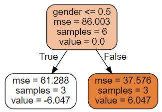
Iteration 2 again tells us that gender matters.

Iteration 3

	name	height	gender	weight	𝑓3	𝑟3	𝛾4	𝑓4	𝑟4
0	Alex	1.6	male	88	75.467259	12.532741	5.427951	76.552849	11.447151
1	Brunei	1.6	female	76	69.781630	6.218370	5.427951	70.867220	5.132780
2	Candy	1.5	female	56	66.866074	-10.866074	-5.427951	65.780484	-9.780484
3	David	1.8	male	73	75.467259	-2.467259	5.427951	76.552849	-3.552849
4	Eric	1.5	male	77	72.551704	4.448296	-5.427951	71.466114	5.533886
5	Felicity	1.4	female	57	66.866074	-9.866074	-5.427951	65.780484	-8.780484

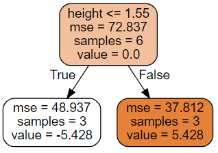
Iteration 3 argues that height is important, too.

Iteration 4

	name	height	gender	weight	𝑓4	𝑟4	𝛾5	𝑓5	𝑟5
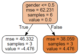
0	Alex	1.6	male	88	76.552849	11.447151	4.476063	77.448062	10.551938
1	Brunei	1.6	female	76	70.867220	5.132780	-4.476063	69.972007	6.027993
2	Candy	1.5	female	56	65.780484	-9.780484	-4.476063	64.885271	-8.885271
3	David	1.8	male	73	76.552849	-3.552849	4.476063	77.448062	-4.448062
4	Eric	1.5	male	77	71.466114	5.533886	4.476063	72.361326	4.638674
5	Felicity	1.4	female	57	65.780484	-8.780484	-4.476063	64.885271	-7.885271

Let’s stop at Iteration 4. And take a look at the loss.

Iteration 4

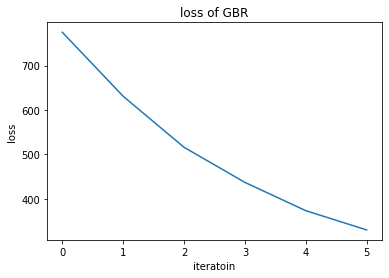
Hope you get the idea.

The code is hosted at my github repo:

https://github.com/EricWebsmith/machine_learning_from_scrach/blob/master/Gradiant_Boosting_Regression.ipynb

Reference:

https://en.wikipedia.org/wiki/Gradient_boosting

https://www.youtube.com/watch?v=3CC4N4z3GJc&list=PLblh5JKOoLUICTaGLRoHQDuF_7q2GfuJF&index=44

https://www.youtube.com/watch?v=2xudPOBz-vs&list=PLblh5JKOoLUICTaGLRoHQDuF_7q2GfuJF&index=45

This article is based on a video from StatQuest, I strongly recommend this Youtube channel.

Author：Eric Websmith

Url: https://ericwebsmith.github.io/2020/04/12/GradientBoostingRegression/

Publish Date: April 12th 2020, 2:44:42 pm

Updated Date: April 19th 2020, 6:53:01 pm

License: We use creativecommons 4.0 license

Next Post

Gradient Boosting Classification from Scratch
Previous Post

Bayesian Optimization

CATALOG

1. The algorithm
2. (Optional) From Gradient Boosting to Gradient Boosting Regression
3. Code
1. 3.1. Step 1 Average
2. 3.2. Step 2 For Loop
4. Reference:



缺失模块。
1、请确保node版本大于6.2
2、在博客根目录（注意不是archer根目录）执行以下命令：
npm i hexo-generator-json-content --save
3、在根目录_config.yml里添加配置：

jsonContent:
  meta: false
  pages: false
  posts:
    title: true
    date: true
    path: true
    text: false
    raw: false
    content: false
    slug: false
    updated: false
    comments: false
    link: false
    permalink: false
    excerpt: false
    categories: true
    tags: true