Gradient Boosting Classification from Scratch

Word count: 2.8kReading time: 17 min

 2020/04/19   Share

The Gradient Boosting (GB) algorithm trains a series of weak learners and each focuses on the errors the previous learners have made and tries to improve it. Together, they make a better prediction.

According to Wikipedia, Gradient boosting is a machine learning technique for regression and classification problems, which produces a prediction model in the form of an ensemble of weak prediction models, typically decision trees. It builds the model in a stage-wise fashion as other boosting methods do, and it generalizes them by allowing optimization of an arbitrary differentiable loss function.

Prerequisite

1. Linear regression and gradient descent
2. Decision Tree
3. Gradient Boosting Regression

After studying this post, you will be able to:

1. Explain gradient boosting algorithm.
2. Explain gradient boosting classification algorithm.
3. Write a gradient boosting classification from scratch

The algorithm

The following plot illustrates the algorithm.

Gradient Boosting Regression

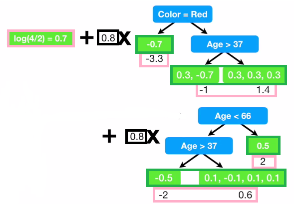
(Picture taken from Youtube channel StatQuest)

From the plot above, the first part is a stump, which is the log of odds of y. We then add several trees to it. In the following trees, the target is not y. Instead, the target is the residual or the true value subtracts the previous prediction.

$residual=true\_value - previous\_prediction$

That is why we say in Gradient Boosting trains a series of weak learners, each focuses on the errors of the previous one. The residual predictions are multiplied by the learning rate (0.1 here) before added to the average.

Here the picture looks more complicated than the one on regression. The purple ones are log of odds (l). The green ones are probabilities. We firstly calculate log of odds of y, instead of average. We then calculate probabilities using log of odds. We build a regression tree. The leaves are colored green. The leaves have residuals. We use the probability residuals to produce log-of-odds residuals or $\gamma$. $\gamma$ is then used to update l. This continues until we are satisfied with the results or we are running out of iterations.

The Steps

Step 1: Calculate the log of odds of y. This is also the first estimation of y. Here $n_1$ is the number of true values and $n_0$ of false values.

$l_0(x)=\log \frac{n_1}{n_0}$

For each $x_i$ , the probability is:

$p_{0i}=\frac{e^{l_{0i}}}{1+e^{l_{0i}}}$

The prediction is:

$f_{0i}=\begin{cases} 0 & p_{0i}<0.5 \\ 1 & p_{0i}>=0.5 \end{cases}$

Step 2 for m in 1 to M:

Step 2.1: Compute so-call pseudo-residuals:

$r_{im}=f_i-p_i$

Step 2.2: Fit a regression tree $t_m(x)$ to pseudo-residuals and create terminal regions (leaves) $R_{jm}$ for $j=1...Jm$
Step 2.3: For each leaf of the tree, there are $p_j$ elements, compute $\gamma$ as following equation.

$\gamma_{im}=\frac{\sum r_{im}}{\sum (1-r_{im-1})(r_{im-1})}$

(In practise, the regression tree will do this for us.)
Step 2.4: Update the log of odds with learning rate $\alpha$:
$l_m(x)=l_{m-1}+\alpha \gamma_m$

For each $x_i$, the probability is:

$p_{mi}=\frac{e^{l_{mi}}}{1+e^{l_{mi}}}$

The prediction is:

$f_{mi}=\begin{cases} 0 & p_{mi}<0.5 \\ 1 & p_{mi}>=0.5 \end{cases}$

Step 3. Output $f_M(x)$

(Optional) From Gradient Boosting to Gradient Boosting Classification

The above knowledge is enough for writing BGR code from scratch. But I want to explain more about gradient boosting. GB is a meta-algorithm that can be applied to both regression and classification. The above one is only a specific form for regression. In the following, I will introduce the general gradient boosting algorithm and deduce GBR from GB.

Let’s first look at the GB steps

The Steps

Input: training set $\{(x_i, y_i)\}_{i=1}^{n}$ , a differentiable loss function $L(y, F(x))$ , number of iterations M

Algorithm:

Step 1: Initialize model with a constant value:

$F_0(x)=\underset{\gamma}{\operatorname{argmin}}\sum_{i=1}^{n}L(y_i, \gamma)$

Step 2 for m in 1 to M:

Step 2.1: Compute so-call pseudo-residuals:
$r_{im}=-[\frac{\partial L(y_i, F(x_i))}{\partial F(x_i)}], {F(x)=F_{m-1}(x)}$
Step 2.2: Fit a weak learner $h_m(x)$ to pseudo-residuals. and create terminal regions $R_{jm}$ , for $j=1...J_m$ .

Step 2.3: For each leaf of the tree, compute $\gamma$ as the following equation.
$\gamma_{jm}=\underset{\gamma}{\operatorname{argmin}}\sum_{x_i \in R_{jm}}^{n}L(y_i, F_{m-1}(x_i)+\gamma)$
Step 2.4: Update the model with learning rate $\alpha$:
$F_m(x)=F_{m-1}+\alpha\gamma_m$

Step 3. Output $F_M(x)$

Lost Function:

To deduce the GB to GBC, I simply define a loss function and solve the loss function in step 1, 2.1 and 2.3. We use Log of Likelihood as the loss function:

$L(y, F(x))=-\sum_{i=1}^{N}(y_i* log(p) + (1-y_i)*log(1-p))$

Since this is a function of probability and we need a function of log of odds( $l$ ), let’s focus on the middle part and transform it into a function of $l$ .

The middle part is:

$-(y*\log(p)+(1-y)*\log(1-p)) \\ =-y * \log(p) - (1-y) * \log(1-p) \\ =-y\log(p)-\log(1-p)+y\log(1-p) \\ =-y(\log(p)-\log(1-p))-\log(1-p) \\ =-y(\log(\frac{p}{1-p}))-\log(1-p) \\ =-y \log(odds)-\log(1-p)$

Since

$\log(1-p)=log(1-\frac{e^{log(odds)}}{1+e^{log(odds)}}) \\ =\log(\frac{1+e^l}{1+e^l}-\frac{e^l}{1+e^l})\\ =\log(\frac{1}{1+e^l}) \\ =\log(1)+\log(1+e^l) \\ =-log(1+e^{\log(odds)})$

We put this to the previous equation:

$-(y*\log(p)+(1-y)*\log(1-p)) \\ =-y\log(odds)+\log(1+e^{\log(odds)}) \\$

Thus, we will have the loss function over log of odds:

$L=-\sum_{i=1}^{N}(y\log(odds)-\log(1+e^{\log(odds)}))$

For Step 1:

Because the lost function is convex and at the lowest point where the derivative is zero, we have the following:

$\frac{\partial L(y, F_0)}{\partial F_0} \\ =-\frac{\partial \sum_{i=1}^{N}(y\log(odds)-\log(1+e^{\log(odds)}))}{\partial log(odds)} \\ =-\sum_{i=1}^{n} y_i+\sum_{i=1}^{N} \frac{\partial log(1+e^{log(odds)})}{\partial log(odds)} \\ =-\sum_{i=1}^{n} y_i+\sum_{i=1}^{N} \frac{1}{1+e^{\log(odds)}} \frac{\partial (1+e^l)}{\partial l} \\ =-\sum_{i=1}^{n} y_i+\sum_{i=1}^{N} \frac{1}{1+e^{\log(odds)}} \frac{\partial (e^l)}{\partial l} \\ =-\sum_{i=1}^{n} y_i+\sum_{i=1}^{N} \frac{e^l}{1+e^l} \\ =-\sum_{i=1}^{n} y_i+N\frac{e^l}{1+e^l}=0$

And We have: (Here p is the real probability)

$\frac{e^l}{1+e^l}=\frac{\sum_{i=1}^{N}y_i}{N}=p \\ e^l=p+p*e^l \\ (1-p)e^l=p \\ e^l=\frac{p}{1-p} \\ \log(odds)=log(\frac{p}{1-p})$

Such that, when log(odds)=log(p/(1-p)) or the probability is the real probability, the lost function is minimized.

For Step 2.1

$r_{im}=-[\frac{\partial L(y_i, F(x_i))}{\partial F(x_i)}]_{F(x)=F_{m-1}(x)}$ $=-[\frac{\partial (-(y_i* log(p)+(1-y_i)*log(1-p)))}{\partial F_{m-1}(x_i)}]_{F(x)=F_{m-1}(x)}$

We have already taken the derivative.

$=y_i-F_{m-1}(x_i)$

For step 2.3:

$\gamma_{jm}=\underset{\gamma}{\operatorname{argmin}}\sum_{x_i \in R_{jm}}^{n}L(y_i, F_{m-1}(x_i)+\gamma)$

I apply the lost function:

$\gamma_{jm} \\ =\underset{\gamma}{\operatorname{argmin}}\sum_{x_i \in R_{jm}}^{n}L(y_i, F_{m-1}(x_i)+\gamma) \\ =\underset{\gamma}{\operatorname{argmin}}\sum_{x_i \in R_{jm}}^{n} (-y_i * (F_{m-1}+\gamma)+\log(1+e^{F_{m-1}+\gamma})) \\$

Let’s focus on the middle part

$-y_i * (F_{m-1}+\gamma)+\log(1+e^{F_{m-1}+\gamma})$

Let’s use Second Order Taylor Polynomial:

$L(y,F+\gamma) \approx L(y, F)+ \frac{d L(y, F+\gamma)\gamma}{d F}+\frac{1}{2} \frac{d^2 L(y, F+\gamma)\gamma^2}{d^2 F}$

Let’s take the derivate:

$\because \frac{d L(y, F+\gamma)}{d\gamma} \approx \frac{d L(y, F)}{d F}+\frac{d^2 L(y, F)\gamma}{d^2 F}=0 \\ \therefore \frac{d L(y, F)}{d F}+\frac{d^2 L(y, F)\gamma}{d^2 F}=0 \\ \therefore \gamma=-\frac{\frac{d L(y, F)}{d F}}{\frac{d^2 L(y, F)}{d^2 F}} \\ \therefore \gamma = \frac{y-p}{\frac{d^2 (-y * l + \log(1+e^l))}{d^2 l}} \\ \therefore \gamma = \frac{y-p}{\frac{d (-y + \frac{e^l}{1+e^l})}{d l}} \\ \therefore \gamma = \frac{y-p}{\frac{d \frac{e^l}{1+e^l}}{d l}} \\$

(The product rule (ab)’=a’ b+a b’)

$\therefore \gamma=\frac{y-p}{\frac{d e^l}{dl} * \frac{1}{1+e^l} - e^l * \frac{d }{d l} \frac{1}{1+e^l}} \\ =\frac{y-p}{\frac{e^l}{1+e^l}-e^l * \frac{1}{(1+e^l)^2} \frac{d}{dl} (1+e^l)} \\ =\frac{y-p}{\frac{e^l}{1+e^l}- \frac{(e^l)^2}{(1+e^l)^2}} \\ =\frac{y-p}{e^l+(e^l)^2-+(e^l)^2} \\ =\frac{y-p}{\frac{e^l}{(1+e^l)^2}} \\ =\frac{y-p}{p(1-p)}$

Now we have

$\gamma = \frac{\sum (y-p)}{\sum p(1-p)}$

Code

Firstly, let’s define a data table as follows:

no	name	likes_popcorn	age	favorite_color	loves_troll2
0	Alex	1	10	Blue	1
1	Brunei	1	90	Green	1
2	Candy	0	30	Blue	0
3	David	1	30	Red	0
4	Eric	0	30	Green	1
5	Felicity	0	10	Blue	1

Step 1

log_of_odds0=np.log(4 / 2)
probability0=np.exp(log_of_odds0)/(np.exp(log_of_odds0)+1)
print(f'the log_of_odds is : {log_of_odds0}')
print(f'the probability is : {probability0}')
predict0=1
print(f'the prediction is : 1')
n_samples=6

loss0=-(y*np.log(probability0)+(1-y)*np.log(1-probability0))

The output is

the log_of_odds is : 0.6931471805599453
the probability is : 0.6666666666666666
the prediction is : 1

Step 2

For Step 2, I define a function called iteration, I will call it several times. Each time we go through from Step 2.1 to Step 2.4.

def iteration(i):
    #step 2.1 calculate the residuals
    residuals[i] = y - probabilities[i]
    #step 2.2 Fit a regression tree
    dt = DecisionTreeRegressor(max_depth=1, max_leaf_nodes=3)
    dt=dt.fit(X, residuals[i])
    
    trees.append(dt.tree_)
    
    #Step 2.3 Calculate gamma
    leaf_indeces=dt.apply(X)
    print(leaf_indeces)
    unique_leaves=np.unique(leaf_indeces)
    n_leaf=len(unique_leaves)
    #for leaf 1
    for ileaf in range(n_leaf):
        
        leaf_index=unique_leaves[ileaf]
        n_leaf=len(leaf_indeces[leaf_indeces==leaf_index])
        previous_probability = probabilities[i][leaf_indeces==leaf_index]
        denominator = np.sum(previous_probability * (1-previous_probability))
        igamma = dt.tree_.value[ileaf+1][0][0] * n_leaf / denominator
        gamma_value[i][ileaf]=igamma
        print(f'for leaf {leaf_index}, we have {n_leaf} related samples. and gamma is {igamma}')

    gamma[i] = [gamma_value[i][np.where(unique_leaves==index)] for index in leaf_indeces]
    #Step 2.4 Update F(x) 
    log_of_odds[i+1] = log_of_odds[i] + learning_rate * gamma[i]

    probabilities[i+1] = np.array([np.exp(odds)/(np.exp(odds)+1) for odds in log_of_odds[i+1]])
    predictions[i+1] = (probabilities[i+1]>0.5)*1.0
    score[i+1]=np.sum(predictions[i+1]==y) / n_samples
    #residuals[i+1] = y - probabilities[i+1]
    loss[i+1]=np.sum(-y * log_of_odds[i+1] + np.log(1+np.exp(log_of_odds[i+1])))
    
    new_df=df.copy()
    new_df.columns=['name', 'popcorn','age','color','y']
    new_df[f'$p_{i}$']=probabilities[i]
    new_df[f'$l_{i}$']=log_of_odds[i]
    new_df[f'$r_{i}$']=residuals[i]
    new_df[f'$\gamma_{i}$']=gamma[i]
    new_df[f'$l_{i+1}$']=log_of_odds[i+1]
    new_df[f'$p_{i+1}$']=probabilities[i+1]
    display(new_df)
    
    dot_data = tree.export_graphviz(dt, out_file=None, filled=True, rounded=True,feature_names=X.columns) 
    graph = graphviz.Source(dot_data) 
    display(graph)

Now Let’s call iteration 0

1	iteration(0)

The output is as follow:

[1 2 2 2 2 1]
for leaf 1, we have 2 related samples. and gamma is 1.5
for leaf 2, we have 4 related samples. and gamma is -0.7499999999999998

no	name	popcorn	age	color	y	𝑝0	𝑙0	𝑟0	𝛾0	𝑙1	𝑝1
0	Alex	1	10	Blue	1	0.666667	0.693147	0.333333	1.50	1.893147	0.869114
1	Brunei	1	90	Green	1	0.666667	0.693147	0.333333	-0.75	0.093147	0.523270
2	Candy	0	30	Blue	0	0.666667	0.693147	-0.666667	-0.75	0.093147	0.523270
3	David	1	30	Red	0	0.666667	0.693147	-0.666667	-0.75	0.093147	0.523270
4	Eric	0	30	Green	1	0.666667	0.693147	0.333333	-0.75	0.093147	0.523270
5	Felicity	0	10	Blue	1	0.666667	0.693147	0.333333	1.50	1.893147	0.869114

tree 0

In Iteration 0, Let’s look at each step.

In Step 2.1, We calculate residuals, that is $y-p_0$.

In step 2.2, we fit a regression tree as above.

In step 2.3, we calculate $\gamma$.

For the first leaf, we have two samples (Alex and Felicity). $\gamma$ is: (1/3+1/3)/((1-2/3)2/3+(1-2/3)2/3)=1.5

For the second leaf, we have four samples. $\gamma$ is:(1/3-2/3-2/3+1/3)/(4(1-2/3)2/3)=-0.75

In Step 2.4, F(x) is updated.

Now, let’s check another iteration

1	iteration(1)

The output is

[1 2 1 1 1 1]
for leaf 1, we have 5 related samples. and gamma is -0.31564962030401844
for leaf 2, we have 1 related samples. and gamma is 1.9110594001952543

	name	popcorn	age	color	y	𝑝1	𝑙1	𝑟1	𝛾1	𝑙2	𝑝2
0	Alex	1	10	Blue	1	0.869114	1.893147	0.130886	-0.315650	1.640627	0.837620
1	Brunei	1	90	Green	1	0.523270	0.093147	0.476730	1.911059	1.621995	0.835070
2	Candy	0	30	Blue	0	0.523270	0.093147	-0.523270	-0.315650	-0.159373	0.460241
3	David	1	30	Red	0	0.523270	0.093147	-0.523270	-0.315650	-0.159373	0.460241
4	Eric	0	30	Green	1	0.523270	0.093147	0.476730	-0.315650	-0.159373	0.460241
5	Felicity	0	10	Blue	1	0.869114	1.893147	0.130886	-0.315650	1.640627	0.837620

tree 1

For Iteration 2, we have two leaves.

For Leaf 1, there are 5 samples. And $\gamma$ is

(0.130886+-0.523270+-0.523270+0.476730+0.130886)/(20.869114(1-0.869114)+30.523270(1-0.523270))=-0.3156498224562022

For Leaf 2, there is only 1 sample. And 𝛾 is 0.476730/(0.523270*(1-0.523270))=1.9110593001700842

Let’s check another iteration

1	iteration(2)

The output:

no	name	popcorn	age	color	y	𝑝2	𝑙2	𝑟2	𝛾2	𝑙3	𝑝3
0	Alex	1	10	Blue	1	0.837620	1.640627	0.162380	1.193858	2.595714	0.930585
1	Brunei	1	90	Green	1	0.835070	1.621995	0.164930	-0.244390	1.426483	0.806353
2	Candy	0	30	Blue	0	0.460241	-0.159373	-0.460241	-0.244390	-0.354885	0.412198
3	David	1	30	Red	0	0.460241	-0.159373	-0.460241	-0.244390	-0.354885	0.412198
4	Eric	0	30	Green	1	0.460241	-0.159373	0.539759	-0.244390	-0.354885	0.412198
5	Felicity	0	10	Blue	1	0.837620	1.640627	0.162380	1.193858	2.595714	0.930585

tree 2

Let’s call iteration 3 and 4

1 2	iteration(3) iteration(4)

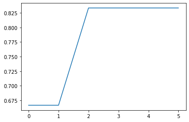
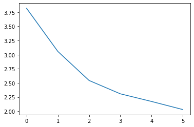
Now, let’s take a look at the loss and accuracy:

Accuracy:

Accuracy

Loss:

Loss

The code is here:

https://github.com/EricWebsmith/machine_learning_from_scrach/blob/master/gradiant_boosting_classification.ipynb

Reference

Gradient Boosting (Wikipedia)

Gradient Boost Part 3: Classification — Youtube StatQuest

Gradient Boost Part 4: Classification Details — Youtube StatQuest

sklearn.tree.DecisionTreeRegressor — scikit-learn 0.21.3 documentation

Understanding the decision tree structure — scikit-learn 0.21.3 documentation

Author：Eric Websmith

Url: https://ericwebsmith.github.io/2020/04/19/GradientBoostingClassification/

Publish Date: April 19th 2020, 5:12:52 pm

Updated Date: April 19th 2020, 6:52:22 pm

License: We use creativecommons 4.0 license

Previous Post

Gradient Boosting Regression from Scratch

CATALOG

1. The algorithm
2. (Optional) From Gradient Boosting to Gradient Boosting Classification
3. Code
4. Reference



缺失模块。
1、请确保node版本大于6.2
2、在博客根目录（注意不是archer根目录）执行以下命令：
npm i hexo-generator-json-content --save
3、在根目录_config.yml里添加配置：

jsonContent:
  meta: false
  pages: false
  posts:
    title: true
    date: true
    path: true
    text: false
    raw: false
    content: false
    slug: false
    updated: false
    comments: false
    link: false
    permalink: false
    excerpt: false
    categories: true
    tags: true